Lesson 2: Signals & Systems (Core Telecom Brain)
Mastering system behaviors for signal processing.
Key Concepts:
- Continuous-time vs discrete-time systems
- LTI systems
- Impulse response
- Sampling theorem (Nyquist)
- Aliasing
- Filtering (LPF, HPF, BPF)
- Analog-to-digital & digital-to-analog conversion
Why It Matters: This forms the “brain” of telecom engineering, enabling design of efficient systems.
Labs/Practice: Implemented filters and sampling in labs; avoided aliasing in digital signal experiments.
Tools Used: MATLAB, Python (SciPy), Simulink.
This is the bridge from pure math (Lesson 1) to actual telecom engineering.
Signals & Systems is where you start thinking like a telecom engineer: how do we process, sample, filter, and digitize signals without losing (or corrupting) the information?
This topic is foundational for digital communications, RF/wireless, cellular networks, and almost every tool & project later (MATLAB, GNU Radio, srsRAN, etc.).
Why Signals & Systems Is the “Core Brain” of Telecom
- Real-world signals are continuous-time analog (voice, radio waves).
- Modern telecom is almost entirely digital after the antenna.
- To go from analog → digital reliably → you need sampling, quantization, filtering, and system analysis.
- Every modulation scheme, equalizer, channel estimator, beamformer, etc., is built on LTI system theory.
- Skip or rush this → you’ll understand what OFDM or QAM does, but not why it survives multipath or noise.
1. Continuous-Time vs Discrete-Time Systems
-
Continuous-time (analog): Signals defined for all real t
Example: s(t) = cos(2π·1000·t)
Systems process them continuously (analog filters, amplifiers). -
Discrete-time (digital): Signals only at integer multiples of sampling period
x[n] = x(n·Tₛ), n = …, -2, -1, 0, 1, 2, …
Processed by DSP chips, FPGAs, software (Python/MATLAB).
Telecom reality
RF front-end is analog/continuous → baseband processing is discrete/digital.
5G NR, Wi-Fi 6, LTE → massive digital signal processing at baseband.
2. LTI Systems (Linear Time-Invariant) — The Golden Assumption
Almost every telecom system we analyze is modeled as LTI:
- Linear: Scaling + superposition
ax₁(t) + bx₂(t) → a·y₁(t) + b·y₂(t) - Time-Invariant: Time shift in input → same time shift in output
Why LTI is huge in telecom
- Filters (channel filters, anti-aliasing, matched filters)
- Channels themselves (in many models, especially AWGN)
- Equalizers, interpolators, beamformers
- Allows powerful math: convolution, frequency response, z-transform/DFT
3. Impulse Response — The DNA of an LTI System
The impulse response h(t) or h[n] completely characterizes an LTI system.
- Input: δ(t) (Dirac delta) → Output: h(t)
-
For any input x(t):
y(t) = x(t) * h(t) (convolution) - Discrete case:
y[n] = ∑ₖ x[k] · h[n-k]
Intuition
h(t) tells you “how the system rings” after a sharp impulse.
Telecom examples
- Matched filter (optimal receiver in AWGN): h(t) = conjugate time-reversed transmitted pulse
- Multipath channel impulse response: multiple delayed copies → causes ISI
→ solved by OFDM or adaptive equalizers
Example: Impulse response of a simple RC low-pass filter (exponential decay — classic “memory” of the filter)
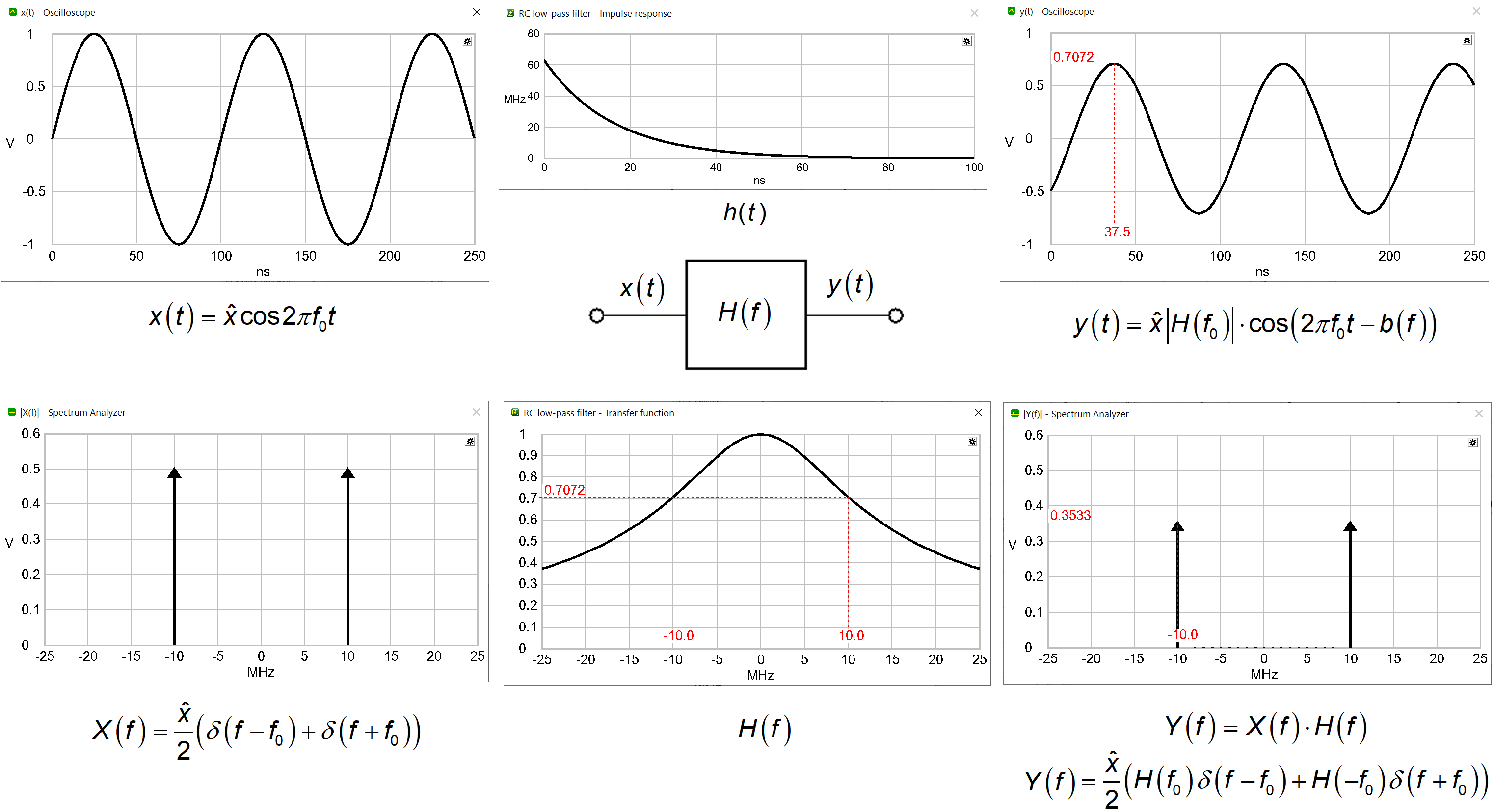
(Exponential decay curve showing how the filter responds to an impulse)
Another view — step response of RC low-pass (shows smoothing effect):
4. Sampling Theorem (Nyquist-Shannon) — The Most Important Rule in Digital Telecom
Theorem
If a signal is bandlimited to maximum frequency fₘₐₓ (no energy above fₘₐₓ),
then sampling at
fₛ ≥ 2·fₘₐₓ
perfectly reconstructs the original signal (using ideal sinc interpolation).
- Nyquist rate = 2·fₘₐₓ
- Nyquist frequency = fₛ / 2
Telecom examples
- Audio: human hearing ~20 kHz → CD uses 44.1 kHz
- 5G baseband: channels up to 100–400 MHz → sampling rates in Gsamples/s in high-end radios
Visual: Proper sampling vs aliasing (sine wave example)

Left: Proper sampling (fₛ > 2×f_max) reconstructs perfectly. Right: Undersampling causes aliasing.
Another clear aliasing demo:
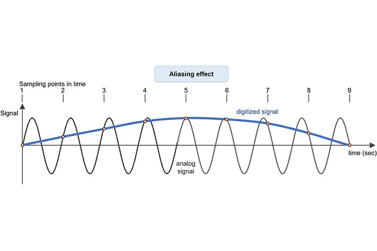
5. Aliasing — The Enemy You Must Understand
When fₛ < 2·fₘₐₓ, frequencies above fₛ/2 fold back into the baseband:
| f_alias = | f - k·fₛ | (for integer k that brings it into [-fₛ/2, fₛ/2]) |
Consequence
High-frequency components masquerade as low-frequency ones → irreversible distortion.
Prevention in real systems
- Always apply anti-aliasing low-pass filter before ADC
Cutoff frequency ≤ fₛ / 2 - In software-defined radio: digital down-conversion + careful decimation
6. Filtering: LPF, HPF, BPF
Filters remove unwanted frequencies.
| Filter Type | Passes | Attenuates | Telecom Use Case |
|---|---|---|---|
| Low-Pass (LPF) | Below cutoff | Above cutoff | Anti-aliasing, baseband signal extraction |
| High-Pass (HPF) | Above cutoff | Below cutoff | Remove DC offset, low-frequency noise |
| Band-Pass (BPF) | Between f₁ and f₂ | Outside the band | Channel selection in receiver |
Example frequency responses (magnitude and phase for Butterworth-style filters)

(Typical LPF roll-off at -3 dB cutoff)

(HPF example — passes high frequencies)
7. Analog-to-Digital & Digital-to-Analog Conversion (ADC / DAC)
ADC chain
- Anti-aliasing LPF
- Sample-and-hold
- Quantization (→ quantization noise)
- Encoding (binary)
DAC: reverse process + reconstruction filter (smooth stair-steps)
Key impairments in telecom
- Quantization noise (increases with fewer bits)
- Aperture jitter (critical at high sampling rates)
- Dynamic range requirements → 12–16 bit ADCs common in base stations
Block diagram of ADC process (with anti-aliasing filter highlighted)
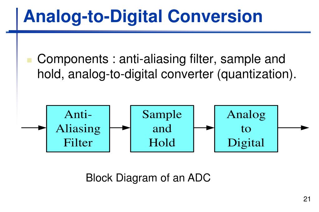
Anti-aliasing filter → Sample & Hold → Quantizer
Another overview:

Tools to Start Using Right Now
- MATLAB —
fft,conv,filter,impz,freqz - Python — NumPy, SciPy.signal, Matplotlib
```python
Quick aliasing demo
import numpy as np import matplotlib.pyplot as plt
t = np.linspace(0, 1, 10000) fs = 100 # sampling rate (too low for some components) f1, f2 = 5, 55 # 55 Hz will alias when fs=100
x = np.sin(2np.pif1t) + 0.7np.sin(2np.pif2*t)
Sampled version
n = np.arange(0, len(t), int(len(t)/(fs*1))) ts = t[n] xs = x[n]
plt.figure(figsize=(12,5)) plt.subplot(121); plt.plot(t, x, label=’continuous’); plt.title(‘Original’); plt.grid(True) plt.subplot(122); plt.stem(ts, xs, label=’sampled @ 100 Hz’); plt.title(‘Aliasing visible’); plt.grid(True) plt.tight_layout(); plt.show()